Categories for Quantum#
Alexis Toumi & Giovanni de Felice
5th May 2021, Tallcat
Categorical quantum mechanics
the miracle of scalars
the way of the dagger
braids and symmetry
compact closed categories
special commutative Frobenius algebras
bialgebras & Hopf algebras
Qubit quantum computing
the circuit model
the ZX-calculus
Applications
optimisation
compilation
extraction
natural language processing
Categorical quantum mechanics#
The traditional formulation of quantum theory happens in \(\mathbf{Hilb}\), the monoidal category of Hilbert spaces and bounded linear maps with the tensor product.
Categorical quantum mechanics (CQM) seeks to make explicit precisely what structure is needed of \(\mathbf{Hilb}\) in order to recover quantum theory.
References:
A categorical semantics of quantum protocols, Abramsky & Coecke (arXiv:0402130)
Categorical quantum mechanics, Abramsky & Coecke (arXiv:0808.1023)
Picturing quantum processes: a first course in quantum theory and diagrammatic reasoning, Coecke & Kissinger (2017)
Categories for quantum theory: an introduction, Heunen & Vicary (2019)
In the process, we get a diagrammatic language for quantum processes.
We also get a new intuition for monoidal categories:
Systems are objects \(A, B\), composition of systems is given by their tensor product \(A \otimes B\).
Processes are arrows \(f : A \to B\), \(g : B \to C\), with their sequential and parallel compositions \(g \circ f\) and \(f \otimes g\).
States are arrows from the unit \(v : 1 \to A\).
Effects are arrows into the unit \(e : A \to 1\).
Scalars are endomorphisms of the unit \(s : 1 \to 1\).
The miracle of scalars#
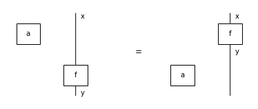
Lemma: Tensoring with a scalar is a natural transformation.
Proof:
[9]:
from discopy.monoidal import Ty, Box
from discopy.drawing import Equation

x, y, z = Ty(*"xyz")
f, g = Box('f', x, y), Box('g', y, z)
a, b, c, d = (Box(x, Ty(), Ty()) for x in 'abcd')

assert a @ x >> f == (f >> a @ y).normal_form()
Equation(a @ x >> f, f >> a @ y).draw(figsize=(5, 2))

Lemma: In a monoidal category, scalars form a commutative monoid.
Proof: Eckmann-Hilton argument.
[10]:
from discopy import drawing

assert (a @ b).interchange(0, 1) == b @ a
assert (a @ b).interchange(0, 1).interchange(0, 1) == a @ b

drawing.to_gif(a @ b, b @ a, loop=True, figsize=(.5, 1), path='../_static/monoidal/Eckmann-Hilton.gif')
[10]:

[10]:
Definition: A monoidal category is enriched in commutative monoids (com.mon. enriched) if every homset is a commutative monoid such that composition and tensor are monoid homomorphisms.
[11]:
from discopy.monoidal import Sum

zero = Sum((), Ty(), Ty())

assert zero + a == Sum((a, )) == a + zero
assert (a + b) + c == a + b + c == a + (b + c)
assert (a + b) @ (c + d) == (a @ c) + (a @ d) + (b @ c) + (b @ d)
assert (a + b) >> (c + d) == (a >> c) + (a >> d) + (b >> c) + (b >> d)
Lemma: In a com.mon. enriched monoidal category, the scalars form a commutative semiring.
Definition: A commutative semiring is a com.mon. enriched monoidal category with one object.
Lemma: Given a commutative semiring \(\mathbb{S}\), the category \(\mathbf{Mat}_\mathbb{S}\) of \(\mathbb{S}\)-valued matrices is monoidal with the Kronecker product.
Lemma: \(\mathbf{FHilb} \simeq \mathbf{Mat}_\mathbb{C}\).
Lemma: \(\mathbf{FRel} \simeq \mathbf{Mat}_\mathbb{B}\).
Com.mon. enrichment allows us to talk about superposition, basis and dimension in an abstract setting.
Definition: Given two states \(v, w : 1 \to A\), their superposition is a linear combination \(a \otimes v + b \otimes w : 1 \to A\) for two scalars \(a, b : 1 \to 1\).
Definition: A basis for \(A\) is a minimal set of states \(\{\vert i \rangle : 1 \to A\}\) such that every state \(w : 1 \to A\) is a linear combination \(w = \sum_i a_i \otimes \vert i \rangle\) for some scalars \(a_i : 1 \to 1\).
Definition: The dimension of a system is the cardinality of its smallest basis.
The way of the dagger#
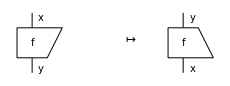
Definition: A dagger is a contravariant involutive identity-on-objects monoidal functor.
In terms of diagrams, the dagger is the vertical reflexion.
We may draw asymmetric boxes to distinguish a generator from its dagger.
[12]:
Equation(f, f[::-1], symbol="$\mapsto$").draw(asymmetry=.25, figsize=(3, 1))

[13]:
from discopy.monoidal import Id
assert Id(x)[::-1] == Id(x)
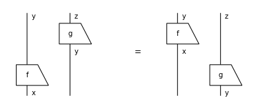
assert (f >> g)[::-1] == g[::-1] >> f[::-1]
assert (f @ g)[::-1].normal_form() == f[::-1] @ g[::-1]
Equation((f @ g)[::-1], f[::-1] @ g[::-1]).draw(figsize=(5, 2))

The dagger allows us to formulate the notion of inner product in an abstract setting.
Definition: The inner product of two states \(w, w' : 1 \to A\) is the scalar \(w^\dagger \circ w' : 1 \to 1\).
Definition: The squared norm of a state \(w : 1 \to A\) is the scalar \(w^\dagger \circ w\). It is normalised when it has norm \(1\), the identity of the monoidal unit.
Definition: Two states \(w, w' : 1 \to A\) are orthogonal when \(w^\dagger \circ w' = 0\).
Definition: An isometry is a norm-preserving process \(f : A \to B\), i.e. \(f^\dagger \circ f = \text{id}_A\).
Definition: A unitary is an isomorphism \(f : A \to B\) with inverse \(f^\dagger\), i.e. \(f^\dagger \circ f = \text{id}_A\) and \(f \circ f^\dagger = \text{id}_B\).
Definition: A basis is orthonormal if \(\langle i | j \rangle = \delta_{ij}\).
It also allows us to talk about quantum measurements, the Born rule and even a simple form of Heisenberg’s uncertainty principle!
Definition: A projector is a process \(p : A \to A\) such that \(p = p^\dagger\) and \(p \circ p = \text{id}_A\).
Example: Take \(w \circ w^\dagger : A \to A\) for any normalised state \(w : 1 \to A\).
Definition: A (projection-valued) measurement is a set of projectors \(\{p_i : A \to A\}\) such that \(\sum p_i = \text{id}_A\).
Example: Take an orthonormal basis \(\{\vert i \rangle\}\) then \(\{\vert i \rangle \langle i \vert\}\) is a measurement.
Lemma: A measurement is a choice of basis and a partition of it.
Definition (Born rule): Given a normalised state \(w : 1 \to A\) and a measurement \(\{p_i : A \to A\}\), the probability of measuring outcome \(i\) and getting the state \(p_i(w)\) as a result is \(P(i \vert w) = w^\dagger \circ p_i \circ w\).
Example: Take \(p_i = v \circ v^\dagger\) then we get the squared amplitude \(P(v \vert w) = \langle w \vert v \rangle^2\).
Definition: Two bases are complementary (a.k.a. mutually unbiased) if \(P(i \vert j) = P(i' \vert j')\) for all \(i, i'\) and \(j, j'\).
Example: Take \(\{\vert 0 \rangle, \vert 1 \rangle\}\) and \(\{\vert + \rangle, \vert - \rangle\}\) the two bases of \(\mathbb{C}^2\) with:
.
Braids and symmetry#
Definition: A (strict) monoidal category is braided if for every objects \(A, B\) we have swaps:

such that


Definition: A braided monoidal category is symmetric if 
or equivalently 
Lemma: In a braided monoidal category, we can prove the Yang-Baxter equation.  Proof: Naturality + Hexagon.
Compact closed categories#
Recall: In a right-rigid monoidal category, for every \(L\) there is a right adjoint \(R\) and a pair of arrows:

such that 
Lemma: In a braided monoidal category, left and right adjoints collapse.
Proof: Define 
Then from naturality we get:

Definition: A compact closed category is a rigid symmetric monoidal category.
Lemma: In a compact closed category, the following equations hold: 
Definition: The transpose of a process is given by: 
Definition: A \(\dagger\) compact closed category is a compact closed category with a dagger, such that swaps are unitaries and
In a \(\dagger\) compact closed category, we get a \(\mathbb{Z}_2 \times \mathbb{Z}_2\) action on processes: 
Compact closed categories allow to formulate the notion of entanglement in an abstract setting.
Definition: A state \(w : 1 \to A \otimes B\) is separable when it can be written as a tensor \(w = v \otimes v'\) for some \(v : 1 \to A\) and \(v' 1 \to B\).
Definition: A state \(w : 1 \to A \otimes B\) is entangled if it is not separable.
Lemma: The cup of a non-trivial system is entangled.
Proof: Suppose the cup is separable, then the identity factors through the unit.

Lemma (Teleportation): 
Proof: 
We can also formulate an abstract version of the no-deleting and no-cloning theorem.
Definition: Deleting is a natural transformation \(e_A : A \to 1\) with \(e_1 = 1\).
Lemma: A monoidal category has deleting if and only if \(1\) is terminal.
Theorem: If a compact closed category has deleting, then it is a preorder.
Proof: Take two parallel arrows \(f, g : A \to B\), then their coname \(\hat f, \hat g : A \otimes B^\star \to 1\) are equal, hence \(f = g\).
Definition: Copying is an commutative, associative natural transformation \(d_A : A \to A \otimes A\) such that:


Lemma: If a braided monoidal category has copying, then:

Proof: 

Theorem: If a compact closed category has copying, then:
Proof: 
Special commutative Frobenius algebras#
Definition: A Frobenius algebra is a pair of a monoid and comonoid such that: 
Definition: A Frobenius algebra is dagger when the dagger of multiplication is comultiplication, and the dagger of unit is counit.
Definition: A \(\dagger\) Frobenius algebra is commutative when its monoid is commutative.
Definition: A \(\dagger\) Frobenius algebra is special when 
Lemma: Frobenius algebras are self-adjoint.
Proof: Define cups and caps 
then
Lemma: Homomorphisms of Frobenius algebras are isomorphisms, with inverse given by

Proof: Suppose \(f\) is a homomorphism of Frobenius algebras. 
Theorem (Spider Fusion): Every connected diagram \(d : A^{\otimes n} \to A^{\otimes m}\) generated by the co/monoid of a Frobenius algebra is equal to a spider-shaped diagram
Proof: By induction, we move all the black comonoid below the white monoid.

Theorem (Artin–Wedderburn): in \(\mathbf{FHilb}\), \(\dagger\) special commutative Frobenius algebras are in one-to-one correspondance with orthonormal bases.
Proof: \(C^\star\) algebra magic.
The correspondance sends a \(\dagger\) SCFA to the basis of copyable states: 
It sends a basis to the Frobenius algebra given by: 
Frobenius algebras not only characterise bases in \(\mathbf{Hilb}\), they also allow us to formulate an abstract notion of phases.
Definition: Given a \(\dagger\)SCFA, a phase is a state \(a : 1 \to A\) such that:

It defines a phase shift map, a.k.a. diagonal unitary matrices: 
Lemma: Phases form a group.

Proof: Associativity and unit follow from that of Frobenius algebras. Define the inverse as follows. 
Then we get 
Bialgebras and Hopf algebras#
Now that we’ve characterised orthonormal bases, we can look at how they interact.
Definition: In a braided monoidal category, a bialgebra is a pair of monoid and comonoid such that: 
Example: In \(\mathbf{Set}\), a bialgebra is a monoid.
Definition: A bialgebra is Hopf when it has an antipode \(s : A \to A\) such that:

Example: In \(\mathbf{Set}\), a Hopf algebra is a group.
Theorem: Two bases are complementary if and only if their corresponding Frobenius algebras obey the Hopf law.
Proof: Define the antipode to be a zebra-snake. 
Then the Hopf law holds if and only if for all \(a\) in the white basis and \(b\) in the black basis:

The right-hand side is equal to \(1\) and the left-hand side simplifies to:

i.e. the probability \(P(a \vert b)\) is constant.
Qubit quantum computing#
The circuit model#
Definition: A gateset is a monoidal signature \(\Sigma\) with one generating object \(\Sigma_0 = \{x\}\) and a monoidal functor \([\![-]\!] : C_\Sigma \to \mathbf{Hilb}\) with \([\![x]\!] = \mathbb{C}^2\) and for all gate \(g \in \Sigma_1\), its evaluation \([\![g]\!]\) is unitary.
Example: Universal gateset \(CX, H, Rx(\theta)\).
Example: Approximately universal \(CX, H, T\).
Definition: A circuit with \(n\)-qubits is a diagram \(d : x^{\otimes n} \to x^{\otimes n}\) in \(C_\Sigma\).
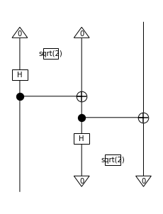
[14]:
from discopy.quantum import Id, CX, H, Ket
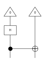
circuit = Ket(0, 0) >> H @ Id(1) >> CX
circuit.draw(figsize=(2, 3))
circuit.eval()

[14]:
Tensor[complex]([0.70710678+0.j, 0. +0.j, 0. +0.j, 0.70710678+0.j], dom=Dim(1), cod=Dim(2, 2))
[14]:
Tensor[complex]([0.70710678+0.j, 0. +0.j, 0. +0.j, 0.70710678+0.j], dom=Dim(1), cod=Dim(2, 2))
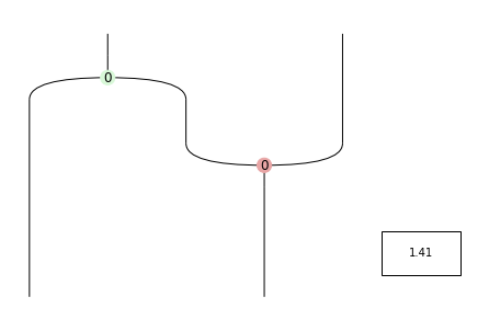
[15]:
Id(1).transpose().draw(figsize=(3, 4))
Id(1).transpose().eval()

[15]:
Tensor[complex]([1.+0.j, 0.+0.j, 0.+0.j, 1.+0.j], dom=Dim(2), cod=Dim(2))
[15]:
Tensor[complex]([1.+0.j, 0.+0.j, 0.+0.j, 1.+0.j], dom=Dim(2), cod=Dim(2))
Finding equations between unitary gates turns out to be difficult, even for two qubits.
Reference: Relations for Clifford+T operators on two qubits, Peter Selinger and Xiaoning Bian (slides)


ZX-calculus#
It turns out that the presentation is much simpler if you axiomatize all of \(\mathbf{FHilb}\) at once, rather than only unitaries. It also allows you to “open the black box” of gates.
[16]:
from discopy.quantum.zx import circuit2zx

circuit2zx(CX).draw()

The axioms are not arcane combinations of black boxes anymore, they come from the interaction of our two friends: \(\dagger\) special commutative Frobenius algebras and Hopf algebras.
Reference: A Near-Optimal Axiomatisation of ZX-Calculus for Pure Qubit Quantum Mechanics, Renaud Vilmart (arXiv:1812.09114)
See also: https://zxcalculus.com/

Theorem: The axioms above are complete for the subcategory of \(\mathbf{Hilb}\) generated by \(\mathbb{C}^2\).
Applications#
Optimization#
Quantum circuits can be simplified using the rules of the ZX calculus.
References:
Optimising Clifford Circuits with Quantomatic, Fagan & Duncan (arXiv:1901.10114)
Graph-theoretic Simplification of Quantum Circuits with the ZX-calculus, Duncan et al. (arXiv:1902.03178)
PyZX: Large Scale Automated Diagrammatic Reasoning, Kissinger, van de Wetering (arXiv:1904.04735)
The structure behind PyZX is a category of cospans of graphs.
Compilation#
We want to compile high-level circuits into low-level gates, and map logical qubits to physical qubits, subject to some architecture constraints on what pairs of qubits can interact.
References:
tket : A Retargetable Compiler for NISQ Devices, Sivarajah et al. (arXiv:2003.10611)
A Generic Compilation Strategy for the Unitary Coupled Cluster Ansatz, Cowtan et al. (arXiv:2007.10515)
Essentially, the data structure behind t|ket> is a free symmetric monoidal category.
Extraction#
Given a ZX diagram, which encodes a measurement-based quantum computation, we want to extract a unitary circuit.
Reference:
There and back again: A circuit extraction tale, Backens et al. (arXiv:2003.01664)
QNLP#
Given the grammar for a sentence, we map each word to circuits and compose them to solve some natural language processing task.
Reference:
Quantum Natural Language Processing on Near-Term Quantum Computers, Meichanetzidis et al. (arXiv:2005.04147)
Grammar-Aware Question-Answering on Quantum Computers, Meichanetzidis et al. (arXiv:2012.03756)