Diagrammatic Differentiation#
Quantum Group Workshop, 26th January 2021
Alexis Toumi, joint work with Richie Yeung and Giovanni de Felice
https://doi.org/10.4204/EPTCS.343.7
1) Parametrised matrices#
Fix a rig \((\mathbb{S}, +, \times, 0, 1)\).
Definition: A matrix \(f \in \mathbf{Mat}_\mathbb{S}(m, n)\) is a function \(f : [m] \times [n] \to \mathbb{S}\) where \([n] = \{0, \dots, n - 1\}\) for \(n \in \mathbb{N}\).
Definition: A parametrised matrix is a function \(f : \mathbb{S} \to \mathbf{Mat}_\mathbb{S}(m, n)\), or equivalently a function-valued matrix \(f \in \mathbf{Mat}_{\mathbb{S} \to \mathbb{S}}(m, n)\).
Example:
[1]:
from discopy.quantum.gates import Rz
from sympy import Expr
from sympy.abc import phi

Rz(phi).array
[1]:
array([[exp(-1.0*I*pi*phi), 0],
       [0, exp(1.0*I*pi*phi)]], dtype=object)
[2]:
(lambda phi: Rz(phi).array)(0.25)
[2]:
array([[0.70710678-0.70710678j, 0.        +0.j        ],
       [0.        +0.j        , 0.70710678+0.70710678j]])
2) Parametrised diagrams#
Fix a monoidal signature \((\Sigma_0, \Sigma_1, \text{dom}, \text{cod} : \Sigma_1 \to \Sigma_0^\star)\) for \(X^\star = \coprod_{n \in \mathbb{N}} X^n\) the free monoid.
Definition: An abstract diagram \(d \in \mathbf{C}_\Sigma(s, t)\) is defined by a list of \(\text{layers}(d) = (\text{left}_0, \text{box}_0, \text{right}_0), \dots, (\text{left}_n, \text{box}_n, \text{right}_n) \in \Sigma_0^\star \times \Sigma_1 \times \Sigma_0^\star\).
Definition: A concrete diagram is an abstract diagram with a monoidal functor \(F : \mathbf{C}_\Sigma \to \mathbf{Mat}_\mathbb{S}\).
Definition: A parametrised diagram is a function \(d : \mathbb{S} \to \mathbf{C}_\Sigma(s, t)\), or equivalently, a diagram with a monoidal functor \(F : \mathbf{C}_\Sigma \to \mathbf{Mat}_{\mathbb{S} \to \mathbb{S}}\).
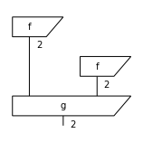
Example:
[3]:
from discopy.tensor import Dim, Box

x, y, z = Dim(1), Dim(2), Dim(2)
f = Box('f', x, y, [phi + 1, -phi * 2])
g = Box('g', y @ y, z, [1, 0, 0, 0, 0, 0, 0, phi ** 2 + 1])

d = f @ f >> g
print(d)
d.draw(figsize=(2, 2))

d.eval(dtype=Expr).array
f >> Dim(2) @ f >> g
[3]:
array([(phi + 1)**2, 4*phi**2*(phi**2 + 1)], dtype=object)
[4]:
d.subs(phi, 0.25).eval(dtype=Expr).array
[4]:
array([1.5625, 0.265625], dtype=object)
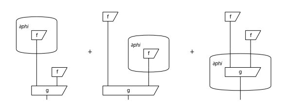
3) Product rule#
We define the gradient of a parametrised matrix \(f \in \mathbf{Mat}_{\mathbb{S} \to \mathbb{S}}(m, n)\) elementwise:
Given a parametrised diagram \(d, F\) we want a new diagram \(\frac{\partial d}{\partial x}\) such that:
We can do this by defining gradients as formal sums of diagrams and using the product rule:
Example:
[5]:
d.grad(phi).draw(figsize=(8, 3), draw_type_labels=False)
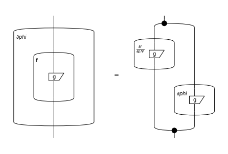
4) Chain rule#
Given an arbitrary function \(f : \mathbb{S} \to \mathbb{S}\), we lift it to matrices by applying it elementwise. Diagrammatically, we represent this as a bubble around a subdiagram.
Gradients of bubbles are then given by the chain rule:
where the elementwise product can be encoded as pre- and post-composition with spiders.
[6]:
g = Box('g', Dim(2), Dim(2), [2 * phi, 0, 0, phi + 1])
f = lambda d: d.bubble(func=lambda x: x ** 2, drawing_name="f")
lhs, rhs = Box.grad(f(g), phi), f(g).grad(phi)

from discopy.drawing import Equation
Equation(lhs, rhs).draw(draw_type_labels=False)
5) Applications#
Gradients of quantum circuits using the parameter shift rule.
Gradients of neural nets and classical post-processing with bubbles.
Gradients of circuit functors for QNLP.